Investigating the Enron Fraud with Machine Learning
Udacity Data Analyst Nanodegree
Overview
In 2000, Enron was one of the largest companies in the United States. By 2002, it had collapsed into bankruptcy due to widespread corporate fraud. In the resulting Federal investigation, a significant amount of typically confidential information entered into the public record, including tens of thousands of emails and detailed financial data for top executives.
Summarize for us the goal of this project and how machine learning is useful in trying to accomplish it. As part of your answer, give some background on the dataset and how it can be used to answer the project question. Were there any outliers in the data when you got it, and how did you handle those?
The goal of this project is to build a person of interest (POI, which means an individual who was indicted, reached a settlement or plea deal with the government, or testified in exchange for prosecution immunity) identifier based on financial and email data made public as a result of the Enron scandal. Machine learning is an excellent tool for this kind of classification task as it can use patterns discovered from labeled data to infer the classes of new observations.
Our dataset combines the public record of Enron emails and financial data with a hand-generated list of POI’s in the fraud case.
Data Exploration
import sys
import cPickle as pickle
import numpy as np
import pandas as pd
import matplotlib.pyplot as plt
import seaborn as sns

from sklearn.cross_validation import train_test_split
from sklearn.pipeline import Pipeline
from sklearn.model_selection import GridSearchCV, StratifiedShuffleSplit, cross_val_score
from sklearn.preprocessing import StandardScaler
from sklearn.decomposition import PCA
from sklearn.feature_selection import SelectKBest
from sklearn.naive_bayes import GaussianNB
from sklearn.svm import SVC
from sklearn.tree import DecisionTreeClassifier
from sklearn.metrics import accuracy_score, precision_score, recall_score, f1_score

sys.path.append("../tools/")

from feature_format import featureFormat, targetFeatureSplit
from tester import dump_classifier_and_data, test_classifier

%matplotlib inline
pd.set_option('display.max_columns', None)

### Load the dictionary containing the dataset
with open("final_project_dataset.pkl", "r") as data_file:
    data_dict = pickle.load(data_file)

# dict to dataframe
df = pd.DataFrame.from_dict(data_dict, orient='index')
df.replace('NaN', np.nan, inplace = True)

df.info()
C:\Users\schil\Anaconda2\lib\site-packages\sklearn\cross_validation.py:44: DeprecationWarning: This module was deprecated in version 0.18 in favor of the model_selection module into which all the refactored classes and functions are moved. Also note that the interface of the new CV iterators are different from that of this module. This module will be removed in 0.20.
  "This module will be removed in 0.20.", DeprecationWarning)


<class 'pandas.core.frame.DataFrame'>
Index: 146 entries, ALLEN PHILLIP K to YEAP SOON
Data columns (total 21 columns):
salary                       95 non-null float64
to_messages                  86 non-null float64
deferral_payments            39 non-null float64
total_payments               125 non-null float64
exercised_stock_options      102 non-null float64
bonus                        82 non-null float64
restricted_stock             110 non-null float64
shared_receipt_with_poi      86 non-null float64
restricted_stock_deferred    18 non-null float64
total_stock_value            126 non-null float64
expenses                     95 non-null float64
loan_advances                4 non-null float64
from_messages                86 non-null float64
other                        93 non-null float64
from_this_person_to_poi      86 non-null float64
poi                          146 non-null bool
director_fees                17 non-null float64
deferred_income              49 non-null float64
long_term_incentive          66 non-null float64
email_address                111 non-null object
from_poi_to_this_person      86 non-null float64
dtypes: bool(1), float64(19), object(1)
memory usage: 24.1+ KB
len(df[df['poi']])
18
There are 146 observations and 21 variables in our dataset - 6 email features, 14 financial features and 1 POI label - and they are divided between 18 POI’s and 128 non-POI’s.
There are a lot of missing values, so, before the data is fed into the machine learning models they are going to be filled by zeros.
Outlier Investigation
df.plot.scatter(x = 'salary', y = 'bonus')
<matplotlib.axes._subplots.AxesSubplot at 0x2d0fb38>
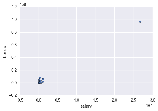
There is a salary bigger than 2.5 *107 🤔. It seems too much even for Enron. Let’s find out whoose is it.
df['salary'].idxmax()
'TOTAL'
This huge salary is the TOTAL of the salaries of the listed employees, so I’m going to remove it.
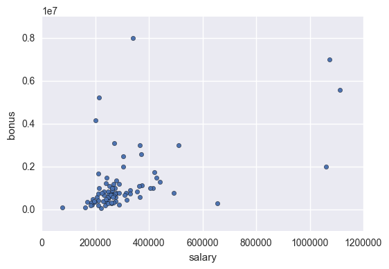
df.drop('TOTAL', inplace = True)
df.plot.scatter(x = 'salary', y = 'bonus')
<matplotlib.axes._subplots.AxesSubplot at 0xc7f6ef0>
Create New Features
What features did you end up using in your POI identifier, and what selection process did you use to pick them? Did you have to do any scaling? Why or why not? As part of the assignment, you should attempt to engineer your own feature that does not come ready-made in the dataset – explain what feature you tried to make, and the rationale behind it. (You do not necessarily have to use it in the final analysis, only engineer and test it.) In your feature selection step, if you used an algorithm like a decision tree, please also give the feature importances of the features that you use, and if you used an automated feature selection function like SelectKBest, please report the feature scores and reasons for your choice of parameter values.
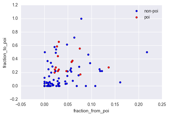
In our dataset we’ve got the number of emails sent to POI’s and received from POI’s for most of the employees. However, if an employee sends or receives a lot of emails in general, it is likely that the quantity of them sent or received from POI’s would be large as well. This is why we are creating these two new features: - fraction of ‘to_messages’ received from a POI; - fraction of ‘from_messages’ sent to a POI.
They can indicate if the majority of an employee’s emails were exchanged with POI’s. In fact, POI’s are grouped together in a scatter plot of the two new features.
df['fraction_from_poi'] = df['from_poi_to_this_person'] / df['to_messages']
df['fraction_to_poi'] = df['from_this_person_to_poi'] / df['from_messages']

ax = df[df['poi'] == False].plot.scatter(x='fraction_from_poi', y='fraction_to_poi', color='blue', label='non-poi')
df[df['poi'] == True].plot.scatter(x='fraction_from_poi', y='fraction_to_poi', color='red', label='poi', ax=ax)
<matplotlib.axes._subplots.AxesSubplot at 0xc9a8898>
Comparing the results for the final chosen model with and without our new engineered features, we get the following results:
| New Features | Accuracy | Precision | Recall | F1 |
|---|---|---|---|---|
| yes | 0.879 | 0.543 | 0.325 | 0.380 |
| no | 0.879 | 0.543 | 0.325 | 0.380 |
Surprisingly the results were the same with and without the two engineered features.
Properly Scale Features
Since we are going to perform a Principal Component Analysis (PCA) to reduce dimensionality later on, and many machine learning models ask for scaled features, a standardization of the features is going to be tested as the first step of our classification pipeline. If it improves the evaluation score of the model then the chosen final model will have this scaling step.
To acomplish it I use the StandardScaler module from scikit learn, which standardizes features by removing the mean and scaling to unit variance.
Intelligently Select Features
The next step in the pipeline is selecting the features that convey the most information to our model.
Leaving some features behind has some advantages, like reducing the noise in the classification, and saving processing time, since there are less features to compute.
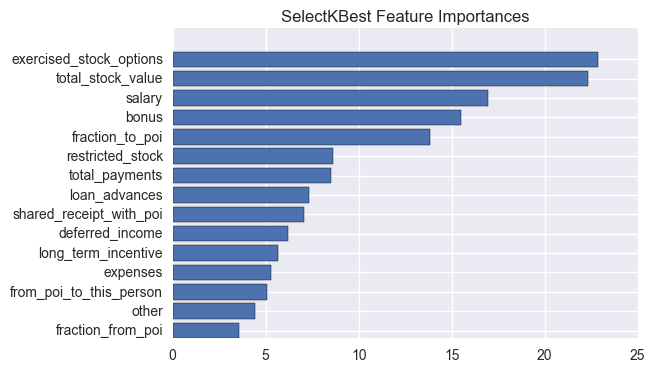
The chosen method was scikit learn’s SelectKBest using f_classif as scoring function. The f_classif function computes the ANOVA F-value between labels and features for classification tasks.
A few feature counts were tested with the aid of a grid search (it will be discussed in a later section), and finally, for the chosen model, 15 most important features were chosen:
| feature | score |
|---|---|
| exercised_stock_options | 22.84690056 |
| total_stock_value | 22.33456614 |
| salary | 16.96091624 |
| bonus | 15.49141455 |
| fraction_to_poi | 13.80595013 |
| restricted_stock | 8.61001147 |
| total_payments | 8.50623857 |
| loan_advances | 7.3499902 |
| shared_receipt_with_poi | 7.06339857 |
| deferred_income | 6.19466529 |
| long_term_incentive | 5.66331492 |
| expenses | 5.28384553 |
| from_poi_to_this_person | 5.05036916 |
| other | 4.42180729 |
| fraction_from_poi | 3.57449894 |
The output of the feature selection was used as input to PCA. The features were projected to a lower dimensional space, reducing dimensionality from 15 features to 6 principal components in our final chosen model.
Pick an Algorithm
What algorithm did you end up using? What other one(s) did you try? How did model performance differ between algorithms?
I ended up using a Gaussian Naïve-Bayes, which scored 0.366984126984 on the nested cross-validation f1. The algorithms tested were: - Gaussian Naïve-Bayes; - Support Vector Machines; - Decision Tree Classifier.
The scores obtained for them are as follows:
| Algorithm | Nested CV f1 |
|---|---|
| Gaussian Naïve-Bayes | 0.366984126984 |
| Support Vector Machines | 0.287132034632 |
| Decision Tree Classifier | 0.228430049483 |
Although the other tested models scored better on other evaluation metrics, it is the nested cross-validation score that best depicts how the model generalizes on unseen data, therefore the Gaussian Naïve-Bayes was the chosen model.
Tune the Algorithm
What does it mean to tune the parameters of an algorithm, and what can happen if you don’t do this well? How did you tune the parameters of your particular algorithm? (Some algorithms do not have parameters that you need to tune – if this is the case for the one you picked, identify and briefly explain how you would have done it for the model that was not your final choice or a different model that does utilize parameter tuning, e.g. a decision tree classifier).
A crucial part of selecting a machine learning algorithm is to adjust it’s parameters in order to maximize the evaluation metrics. If the parameters are not properly tuned, the algorithm can underfit or overfit the data, hence producing suboptimal results.
To tune the algorithms, I used the GridSearchCV tool provided in scikit learn. It exhaustively searches for the best parameters between the ones specified in an array of possibilities. The parameters are chosen in order to optimize the chosen scoring function, in our case, f1 (the evaluation metrics will be better addressed on the ‘Usage of Evaluation Metrics’ section).
Validation Strategy
What is validation, and what’s a classic mistake you can make if you do it wrong? How did you validate your analysis?
Validation in machine learning consists of evaluating a model using data that was not touched during the training process. A classic mistake is to ignore this rule, hence obtaining overly optimistic results due to overfitting the training data, but very poor performance on unseen data.
It is a good practice to separate data in three parts: training, cross-validation and test sets. The model is tuned to maximize the evaluation score on the cross-validation set, and then the final model efficiency is measured on the test set.
Since there are too few observations for us to train and test the algorithms, in order to extract the most information from the data, the selected strategy to validate our model was a Nested Stratified Shuffle Split Cross-Validation.
In this strategy effectively uses a series of train/validation/test set splits. In the inner loop, the score is approximately maximized by fitting a model to each training set, and then directly maximized in selecting (hyper)parameters over the validation set. In the outer loop, generalization error is estimated by averaging test set scores over several dataset splits. All sets are picked randomly, but keeping the same proportion of class labels.
Usage of Evaluation Metrics
Give at least 2 evaluation metrics and your average performance for each of them. Explain an interpretation of your metrics that says something human-understandable about your algorithm’s performance.
For classification algorithms, some of the most common evaluation metrics are accuracy, precision, recall and the f1 score.
Accuracy shows the ratio between right classifications and the total number of predicted labels. Since the POI/non-POI distribution is very uneven, accuracy does not mean much. A model that predicts always non-POI’s would get an accuracy of 87.6%, which is an apparently good score for a terrible classifier.
Precision is the ratio of right classifications over all observations with a given predicted label. For example, the ratio of true POI’s over all predicted POI’s.
Recall is the ratio of right classifications over all observations that are truly of a given class. For example, the ratio of observations correctly labeled POI over all true POI’s.
F1 is a way of balance precision and recall, and is given by the following formula:
$$F1 = 2 * (precision * recall) / (precision + recall)$$
For the final selected model, the average scores were the following:
| Model | Accuracy | Precision | Recall | F1 |
|---|---|---|---|---|
| GaussianNB | 0.879310344828 | 0.543333333333 | 0.325 | 0.38 |
Additional Code
### The first feature must be "poi".
features_list = ['poi', 'salary', 'bonus', 'long_term_incentive', 'deferred_income', 'deferral_payments',
                 'loan_advances', 'other', 'expenses', 'director_fees', 'total_payments',
                 'exercised_stock_options', 'restricted_stock', 'restricted_stock_deferred',
                 'total_stock_value', 'to_messages', 'from_messages', 'from_this_person_to_poi',
                 'from_poi_to_this_person', 'shared_receipt_with_poi', 'fraction_from_poi', 'fraction_to_poi']

### Load the dictionary containing the dataset
filled_df = df.fillna(value='NaN') # featureFormat expects 'NaN' strings
data_dict = filled_df.to_dict(orient='index')

### Store to my_dataset for easy export below.
my_dataset = data_dict

### Extract features and labels from dataset for local testing
data = featureFormat(my_dataset, features_list, sort_keys = True)
y, X = targetFeatureSplit(data)
X = np.array(X)
y = np.array(y)

### Cross-validation
sss = StratifiedShuffleSplit(n_splits=10, test_size=0.2, random_state=42)

SCALER = [None, StandardScaler()]
SELECTOR__K = [10, 13, 15, 18, 'all']
REDUCER__N_COMPONENTS = [2, 4, 6, 8, 10]
def evaluate_model(grid, X, y, cv):
    nested_score = cross_val_score(grid, X=X, y=y, cv=cv, n_jobs=-1)
    print "Nested f1 score: {}".format(nested_score.mean())

    grid.fit(X, y)
    print "Best parameters: {}".format(grid.best_params_)

    cv_accuracy = []
    cv_precision = []
    cv_recall = []
    cv_f1 = []
    for train_index, test_index in cv.split(X, y):
        X_train, X_test = X[train_index], X[test_index]
        y_train, y_test = y[train_index], y[test_index]

        grid.best_estimator_.fit(X_train, y_train)
        pred = grid.best_estimator_.predict(X_test)

        cv_accuracy.append(accuracy_score(y_test, pred))
        cv_precision.append(precision_score(y_test, pred))
        cv_recall.append(recall_score(y_test, pred))
        cv_f1.append(f1_score(y_test, pred))

    print "Mean Accuracy: {}".format(np.mean(cv_accuracy))
    print "Mean Precision: {}".format(np.mean(cv_precision))
    print "Mean Recall: {}".format(np.mean(cv_recall))
    print "Mean f1: {}".format(np.mean(cv_f1))
Gaussian Naïve-Bayes
### comment to perform a full hyperparameter search
# SCALER = [None]
# SELECTOR__K = [15]
# REDUCER__N_COMPONENTS = [6]
###################################################

pipe = Pipeline([
        ('scaler', StandardScaler()),
        ('selector', SelectKBest()),
        ('reducer', PCA(random_state=42)),
        ('classifier', GaussianNB())
    ])

param_grid = {
    'scaler': SCALER,
    'selector__k': SELECTOR__K,
    'reducer__n_components': REDUCER__N_COMPONENTS
}

gnb_grid = GridSearchCV(pipe, param_grid, scoring='f1', cv=sss)

evaluate_model(gnb_grid, X, y, sss)

test_classifier(gnb_grid.best_estimator_, my_dataset, features_list)
Nested f1 score: 0.366984126984


C:\Users\schil\Anaconda2\lib\site-packages\sklearn\metrics\classification.py:1113: UndefinedMetricWarning: F-score is ill-defined and being set to 0.0 due to no predicted samples.
  'precision', 'predicted', average, warn_for)


Best parameters: {'reducer__n_components': 6, 'selector__k': 15, 'scaler': None}
Mean Accuracy: 0.879310344828
Mean Precision: 0.543333333333
Mean Recall: 0.325
Mean f1: 0.38


C:\Users\schil\Anaconda2\lib\site-packages\sklearn\metrics\classification.py:1113: UndefinedMetricWarning: Precision is ill-defined and being set to 0.0 due to no predicted samples.
  'precision', 'predicted', average, warn_for)
C:\Users\schil\Anaconda2\lib\site-packages\sklearn\feature_selection\univariate_selection.py:113: UserWarning: Features [5] are constant.
  UserWarning)


Pipeline(steps=[('scaler', None), ('selector', SelectKBest(k=15, score_func=<function f_classif at 0x000000000C5869E8>)), ('reducer', PCA(copy=True, iterated_power='auto', n_components=6, random_state=42,
  svd_solver='auto', tol=0.0, whiten=False)), ('classifier', GaussianNB(priors=None))])
    Accuracy: 0.85733   Precision: 0.44868  Recall: 0.30600 F1: 0.36385 F2: 0.32678
    Total predictions: 15000    True positives:  612    False positives:  752   False negatives: 1388   True negatives: 12248
kbest = gnb_grid.best_estimator_.named_steps['selector']

features_array = np.array(features_list)
features_array = np.delete(features_array, 0)
indices = np.argsort(kbest.scores_)[::-1]
k_features = kbest.get_support().sum()

features = []
for i in range(k_features):
    features.append(features_array[indices[i]])

features = features[::-1]
scores = kbest.scores_[indices[range(k_features)]][::-1]

plt.barh(range(k_features), scores)
plt.yticks(np.arange(0.4, k_features), features)
plt.title('SelectKBest Feature Importances')
plt.show()
# Without the engineered features
# removing the 2 last columns
X_2 = np.delete(X, -1, 1)
X_2 = np.delete(X_2, -1, 1)

evaluate_model(gnb_grid, X_2, y, sss)
Nested f1 score: 0.345079365079
Best parameters: {'reducer__n_components': 6, 'selector__k': 13, 'scaler': None}
Mean Accuracy: 0.879310344828
Mean Precision: 0.543333333333
Mean Recall: 0.325
Mean f1: 0.38
Support Vector Machine Classifier
C_PARAM = np.logspace(-2, 3, 6)
GAMMA_PARAM = np.logspace(-4, 1, 6)
CLASS_WEIGHT = ['balanced', None]
KERNEL = ['rbf', 'sigmoid']

### comment to perform a full hyperparameter search
# SCALER = [StandardScaler()]
# SELECTOR__K = [18]
# REDUCER__N_COMPONENTS = [10]
# C_PARAM = [100]
# GAMMA_PARAM = [.01]
# CLASS_WEIGHT = ['balanced']
# KERNEL = ['sigmoid']
###################################################

pipe = Pipeline([
        ('scaler', StandardScaler()),
        ('selector', SelectKBest()),
        ('reducer', PCA(random_state=42)),
        ('classifier', SVC())
    ])

param_grid = {
    'scaler': SCALER,
    'selector__k': SELECTOR__K,
    'reducer__n_components': REDUCER__N_COMPONENTS,
    'classifier__C': C_PARAM,
    'classifier__gamma': GAMMA_PARAM,
    'classifier__class_weight': CLASS_WEIGHT,
    'classifier__kernel': KERNEL
}

svc_grid = GridSearchCV(pipe, param_grid, scoring='f1', cv=sss)

evaluate_model(svc_grid, X, y, sss)

test_classifier(svc_grid.best_estimator_, my_dataset, features_list)
Nested f1 score: 0.287132034632
Best parameters: {'reducer__n_components': 10, 'selector__k': 18, 'scaler': StandardScaler(copy=True, with_mean=True, with_std=True), 'classifier__class_weight': 'balanced', 'classifier__gamma': 0.01, 'classifier__kernel': 'sigmoid', 'classifier__C': 100.0}
Mean Accuracy: 0.827586206897
Mean Precision: 0.460887445887
Mean Recall: 0.8
Mean f1: 0.566651681652
Pipeline(steps=[('scaler', StandardScaler(copy=True, with_mean=True, with_std=True)), ('selector', SelectKBest(k=18, score_func=<function f_classif at 0x000000000C5869E8>)), ('reducer', PCA(copy=True, iterated_power='auto', n_components=10, random_state=42,
  svd_solver='auto', tol=0.0, whiten=False)), ('cla...,
  max_iter=-1, probability=False, random_state=None, shrinking=True,
  tol=0.001, verbose=False))])
    Accuracy: 0.76920   Precision: 0.33595  Recall: 0.74850 F1: 0.46375 F2: 0.60092
    Total predictions: 15000    True positives: 1497    False positives: 2959   False negatives:  503   True negatives: 10041
Decision Tree Classifier
CRITERION = ['gini', 'entropy']
SPLITTER = ['best', 'random']
MIN_SAMPLES_SPLIT = [2, 4, 6, 8]
CLASS_WEIGHT = ['balanced', None]

### comment to perform a full hyperparameter search
# SCALER = [StandardScaler()]
# SELECTOR__K = [18]
# REDUCER__N_COMPONENTS = [2]
# CRITERION = ['gini']
# SPLITTER = ['random']
# MIN_SAMPLES_SPLIT = [8]
# CLASS_WEIGHT = ['balanced']
###################################################

pipe = Pipeline([
        ('scaler', StandardScaler()),
        ('selector', SelectKBest()),
        ('reducer', PCA(random_state=42)),
        ('classifier', DecisionTreeClassifier())
    ])

param_grid = {
    'scaler': SCALER,
    'selector__k': SELECTOR__K,
    'reducer__n_components': REDUCER__N_COMPONENTS,
    'classifier__criterion': CRITERION,
    'classifier__splitter': SPLITTER,
    'classifier__min_samples_split': MIN_SAMPLES_SPLIT,
    'classifier__class_weight': CLASS_WEIGHT,
}

tree_grid = GridSearchCV(pipe, param_grid, scoring='f1', cv=sss)

evaluate_model(tree_grid, X, y, sss)

test_classifier(tree_grid.best_estimator_, my_dataset, features_list)
Nested f1 score: 0.228430049483
Best parameters: {'reducer__n_components': 4, 'selector__k': 15, 'scaler': StandardScaler(copy=True, with_mean=True, with_std=True), 'classifier__min_samples_split': 8, 'classifier__class_weight': 'balanced', 'classifier__splitter': 'random', 'classifier__criterion': 'gini'}
Mean Accuracy: 0.758620689655
Mean Precision: 0.325331890332
Mean Recall: 0.425
Mean f1: 0.321083916084
Pipeline(steps=[('scaler', StandardScaler(copy=True, with_mean=True, with_std=True)), ('selector', SelectKBest(k=15, score_func=<function f_classif at 0x000000000C5869E8>)), ('reducer', PCA(copy=True, iterated_power='auto', n_components=4, random_state=42,
  svd_solver='auto', tol=0.0, whiten=False)), ('clas...=8, min_weight_fraction_leaf=0.0,
            presort=False, random_state=None, splitter='random'))])
    Accuracy: 0.73587   Precision: 0.24677  Recall: 0.47800 F1: 0.32550 F2: 0.40256
    Total predictions: 15000    True positives:  956    False positives: 2918   False negatives: 1044   True negatives: 10082