Exploring and Summarizing White Wine Data with R
Udacity Data Analyst Nanodegree
Project Overview
This report explores a dataset containing attributes for 4898 instances of the Portuguese “Vinho Verde” white wine.
The attributes are the following:
- fixed acidity (tartaric acid - g / dm3): most acids involved with wine are fixed or nonvolatile (do not evaporate readily).
- volatile acidity (acetic acid - g / dm3): the amount of acetic acid in wine, which at too high of levels can lead to an unpleasant, vinegar taste.
- citric acid (g / dm3): found in small quantities, citric acid can add ‘freshness’ and flavor to wines.
- residual sugar (g / dm3): the amount of sugar remaining after fermentation stops. It’s rare to find wines with less than 1 g / dm3 and wines with more than 45 g / dm3 are considered sweet.
- chlorides (sodium chloride - g / dm3): the amount of salt in the wine.
- free sulfur dioxide (mg / dm3): the free form of SO2 exists in equilibrium between molecular SO2 (as a dissolved gas) and bisulfite ion. It prevents microbial growth and the oxidation of wine.
- total sulfur dioxide (mg / dm3): amount of free and bound forms of S02. In low concentrations, SO2 is mostly undetectable in wine, but at free SO2 concentrations over 50 ppm, SO2 becomes evident in the nose and taste of wine.
- density (g / cm3): the density of wine is close to that of water depending on the percent alcohol and sugar content.
- pH - describes how acidic or basic a wine is on a scale from 0 (very acidic) to 14 (very basic); most wines are between 3-4 on the pH scale.
- sulphates (potassium sulphate - g / dm3): a wine additive which can contribute to sulfur dioxide gas (S02) levels, wich acts as an antimicrobial and antioxidant.
- alcohol (% by volume) - the percent alcohol content of the wine.
- quality: score between 0 and 10 (based on sensory data).
Univariate Plots Section
## 'data.frame':    4898 obs. of  12 variables:
##  $ fixed.acidity       : num  7 6.3 8.1 7.2 7.2 8.1 6.2 7 6.3 8.1 ...
##  $ volatile.acidity    : num  0.27 0.3 0.28 0.23 0.23 0.28 0.32 0.27 0.3 0.22 ...
##  $ citric.acid         : num  0.36 0.34 0.4 0.32 0.32 0.4 0.16 0.36 0.34 0.43 ...
##  $ residual.sugar      : num  20.7 1.6 6.9 8.5 8.5 6.9 7 20.7 1.6 1.5 ...
##  $ chlorides           : num  0.045 0.049 0.05 0.058 0.058 0.05 0.045 0.045 0.049 0.044 ...
##  $ free.sulfur.dioxide : num  45 14 30 47 47 30 30 45 14 28 ...
##  $ total.sulfur.dioxide: num  170 132 97 186 186 97 136 170 132 129 ...
##  $ density             : num  1.001 0.994 0.995 0.996 0.996 ...
##  $ pH                  : num  3 3.3 3.26 3.19 3.19 3.26 3.18 3 3.3 3.22 ...
##  $ sulphates           : num  0.45 0.49 0.44 0.4 0.4 0.44 0.47 0.45 0.49 0.45 ...
##  $ alcohol             : num  8.8 9.5 10.1 9.9 9.9 10.1 9.6 8.8 9.5 11 ...
##  $ quality             : int  6 6 6 6 6 6 6 6 6 6 ...

##  fixed.acidity    volatile.acidity  citric.acid     residual.sugar
##  Min.   : 3.800   Min.   :0.0800   Min.   :0.0000   Min.   : 0.600
##  1st Qu.: 6.300   1st Qu.:0.2100   1st Qu.:0.2700   1st Qu.: 1.700
##  Median : 6.800   Median :0.2600   Median :0.3200   Median : 5.200
##  Mean   : 6.855   Mean   :0.2782   Mean   :0.3342   Mean   : 6.391
##  3rd Qu.: 7.300   3rd Qu.:0.3200   3rd Qu.:0.3900   3rd Qu.: 9.900
##  Max.   :14.200   Max.   :1.1000   Max.   :1.6600   Max.   :65.800
##    chlorides       free.sulfur.dioxide total.sulfur.dioxide
##  Min.   :0.00900   Min.   :  2.00      Min.   :  9.0
##  1st Qu.:0.03600   1st Qu.: 23.00      1st Qu.:108.0
##  Median :0.04300   Median : 34.00      Median :134.0
##  Mean   :0.04577   Mean   : 35.31      Mean   :138.4
##  3rd Qu.:0.05000   3rd Qu.: 46.00      3rd Qu.:167.0
##  Max.   :0.34600   Max.   :289.00      Max.   :440.0
##     density             pH          sulphates         alcohol
##  Min.   :0.9871   Min.   :2.720   Min.   :0.2200   Min.   : 8.00
##  1st Qu.:0.9917   1st Qu.:3.090   1st Qu.:0.4100   1st Qu.: 9.50
##  Median :0.9937   Median :3.180   Median :0.4700   Median :10.40
##  Mean   :0.9940   Mean   :3.188   Mean   :0.4898   Mean   :10.51
##  3rd Qu.:0.9961   3rd Qu.:3.280   3rd Qu.:0.5500   3rd Qu.:11.40
##  Max.   :1.0390   Max.   :3.820   Max.   :1.0800   Max.   :14.20
##     quality
##  Min.   :3.000
##  1st Qu.:5.000
##  Median :6.000
##  Mean   :5.878
##  3rd Qu.:6.000
##  Max.   :9.000
Main feature of interest: Quality
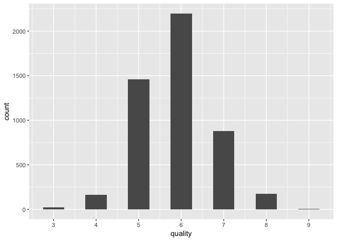
##    Min. 1st Qu.  Median    Mean 3rd Qu.    Max.
##   3.000   5.000   6.000   5.878   6.000   9.000
Quality follows a normal-like distribution with discrete integer values.
Regarding acidity
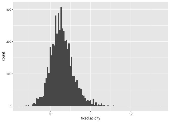
##    Min. 1st Qu.  Median    Mean 3rd Qu.    Max.
##   3.800   6.300   6.800   6.855   7.300  14.200
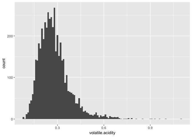
##    Min. 1st Qu.  Median    Mean 3rd Qu.    Max.
##  0.0800  0.2100  0.2600  0.2782  0.3200  1.1000
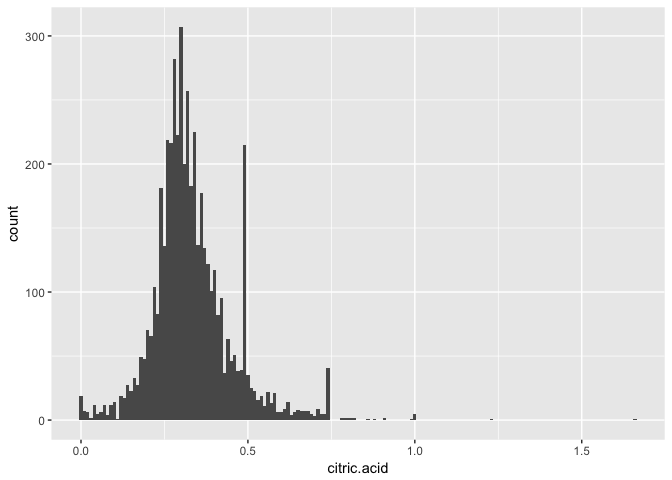
##    Min. 1st Qu.  Median    Mean 3rd Qu.    Max.
##  0.0000  0.2700  0.3200  0.3342  0.3900  1.6600
There is an interesting peak at .49 and a smaller one at .74g / dm3. This suggests me that maybe a standard amount of citric acid is added to some of the wines.
## Min. 1st Qu. Median Mean 3rd Qu. Max.
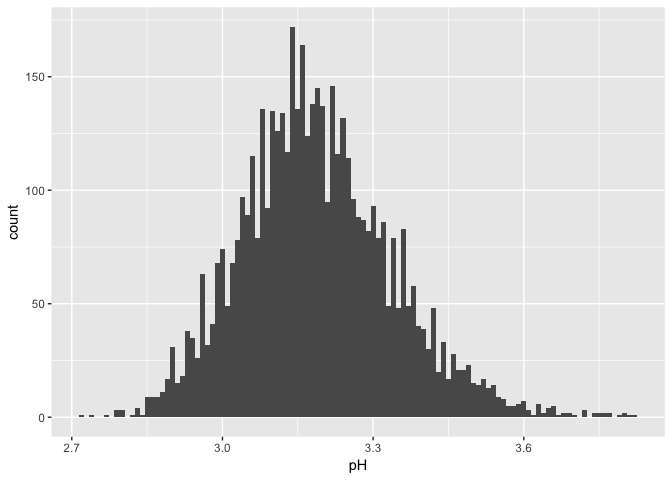
## 2.720 3.090 3.180 3.188 3.280 3.820
The pH shows a bell shaped distribution. I wonder how it relates individually to the concentrations of acids.
Regarding SO2
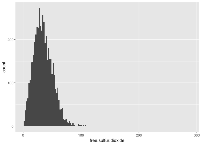
##    Min. 1st Qu.  Median    Mean 3rd Qu.    Max.
##    2.00   23.00   34.00   35.31   46.00  289.00
Free sulfur dioxide has some extreme outliers to the right of the curve.
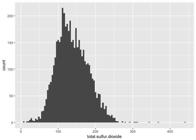
##    Min. 1st Qu.  Median    Mean 3rd Qu.    Max.
##     9.0   108.0   134.0   138.4   167.0   440.0
wines$bound.sulfur.dioxide <- with(wines,
                                   total.sulfur.dioxide - free.sulfur.dioxide)
wines$sulfur.dioxide.ratio <- with(wines,
                                   free.sulfur.dioxide / bound.sulfur.dioxide)
I created a bound sulfur dioxide variable by subtracting the free from the total sulfur dioxide. Then I created a feature consisting of the ratio between the free and bound sulfur dioxide present in the wine.
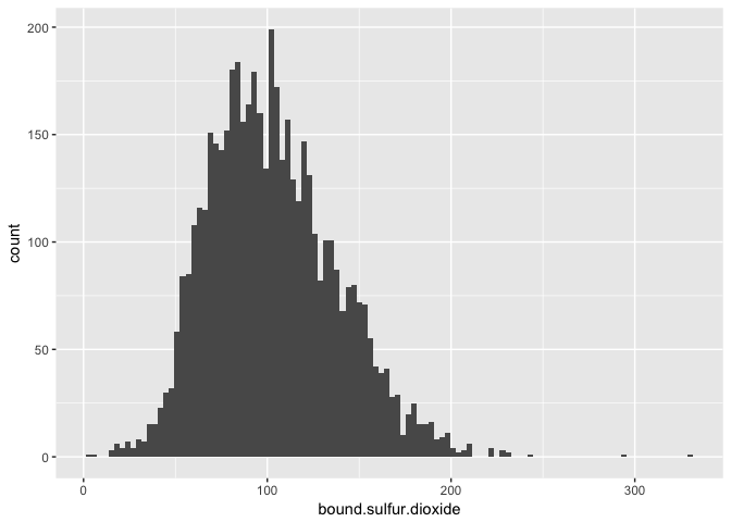
##    Min. 1st Qu.  Median    Mean 3rd Qu.    Max.
##     4.0    78.0   100.0   103.1   125.0   331.0
It looks very similar to the total sulfur dioxide.
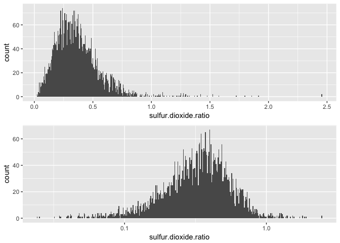
##    Min. 1st Qu.  Median    Mean 3rd Qu.    Max.
## 0.02419 0.23600 0.33990 0.36750 0.46150 2.45500
I transformed the scale to log10 to better visualize the distribution. Maybe it will be useful when trying to predict the quality, or even give us some insight about the data.
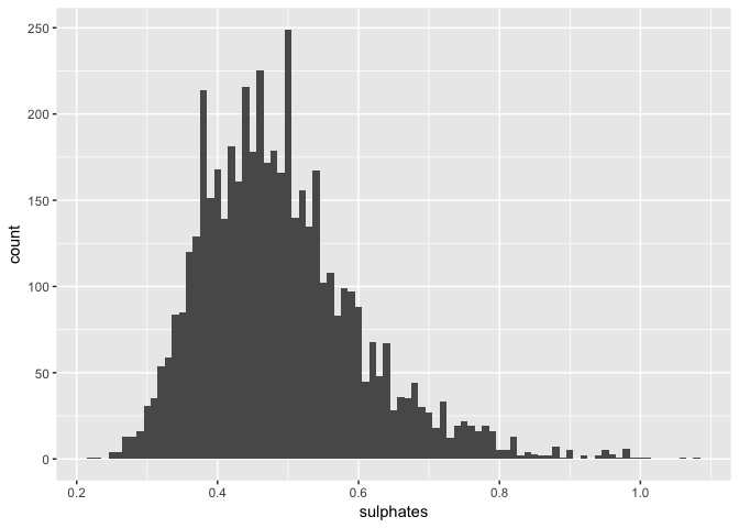
##    Min. 1st Qu.  Median    Mean 3rd Qu.    Max.
##  0.2200  0.4100  0.4700  0.4898  0.5500  1.0800
Sulphates are a little positively skewed. Since it can contribute to sulfur dioxide levels, it can be valuable to plot relations between them.
Other attributes
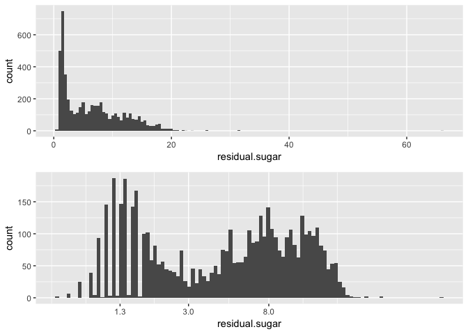
##    Min. 1st Qu.  Median    Mean 3rd Qu.    Max.
##   0.600   1.700   5.200   6.391   9.900  65.800
I transformed the residual sugar to a log10 scale to better visualize its distribution. The transformed variable appears bimodal, with peaks around 1.3 and 8.
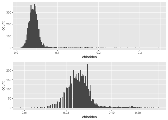
##    Min. 1st Qu.  Median    Mean 3rd Qu.    Max.
## 0.00900 0.03600 0.04300 0.04577 0.05000 0.34600
I transformed the long tail distribution with a log10 scale so it could be better visualized. After the transformation, the chlorides histogram appears normal, with some outliers on the right side of the curve.
## Min. 1st Qu. Median Mean 3rd Qu. Max.
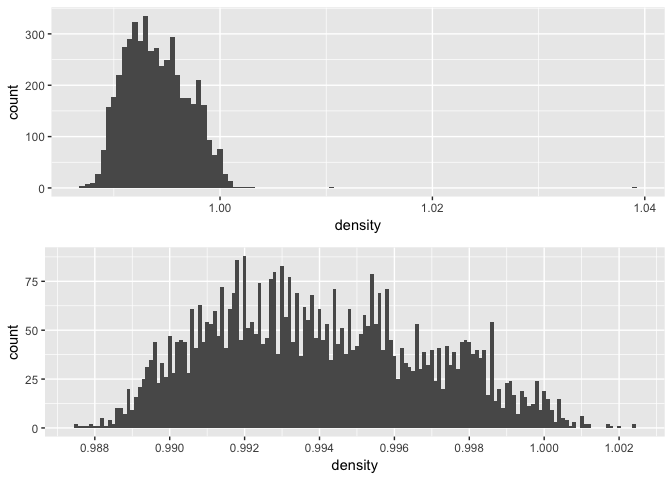
## 0.9871 0.9917 0.9937 0.9940 0.9961 1.0390
Most of the density values are between .99 and 1.00 g / cm3, but there are some outliers near 1.01 and 1.04.
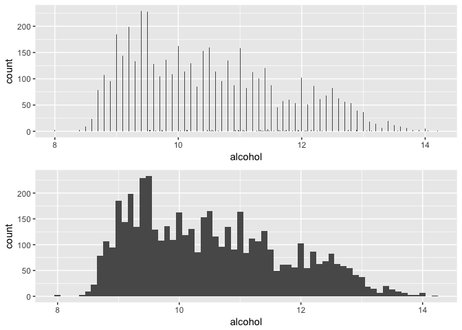
##    Min. 1st Qu.  Median    Mean 3rd Qu.    Max.
##    8.00    9.50   10.40   10.51   11.40   14.20
Alcohol presents mostly discrete values, with intervals of .1%. There are a few exceptions though.
Univariate Analysis
What is the structure of your dataset?
There are 11 variables representing physicochemical measurements and 1 variable representing the median of at least 3 evaluations of quality made by wine experts, varying from 0 (very bad) to 10 (very excellent).
What is/are the main feature(s) of interest in your dataset?
Quality is the main feature of interest. The objective of the analysis is to determine the features that influence wine quality the most, and then building a predictive model of quality using these variables.
What other features in the dataset do you think will help support your investigation into your feature(s) of interest?
Most features have an aproximately normal distribution, just like the quality variable. It makes it hard to guess which features will have a greater impact on the prediction of quality.
Did you create any new variables from existing variables in the dataset?
I created the “sulfur.dioxide.ratio”, which consists of the ratio between “free.sulfur.dioxide” and “total.sulfur.dioxide”.
Of the features you investigated, were there any unusual distributions? Did you perform any operations on the data to tidy, adjust, or change the form of the data? If so, why did you do this?
The distribution of citric acid presented two unusual peaks which standed out of an otherwise normal distribution.
I preformed a log transformation on the residual sugar and chlorides distributions, because they were very skewed, and the transformations allowed better visualizations of the data.
Bivariate Plots Section
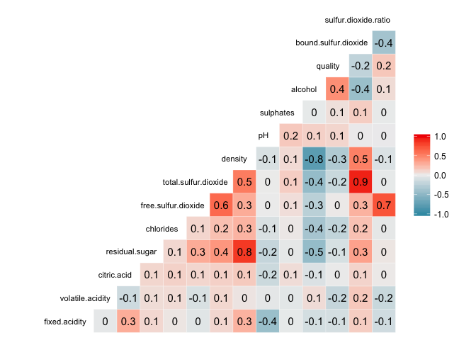
This correlation matrix naturally shows strong correlations between free sulfur dioxide, total sulfur dioxide and the constructed variables bound sulfur dioxide and sulfur dioxide ratio.
It also shows interesting relations between residual.sugar vs density and alcohol vs density.
Density, residual sugar and alcohol
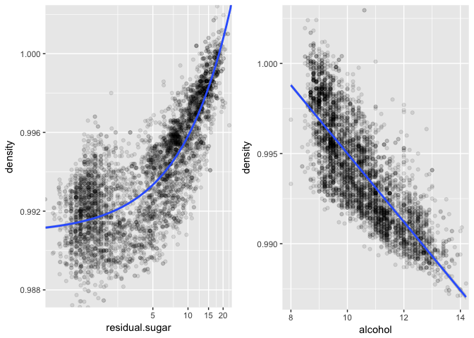
Density varies aproximately linearly with residual sugar (positive correlation) and with alcohol (negative correlation). It makes sense, taking into account the fermentation process of wine, in which sugar is consumed to generate alcohol. And since the residual sugar is more dense than alcohol, this inverse relation is presented.
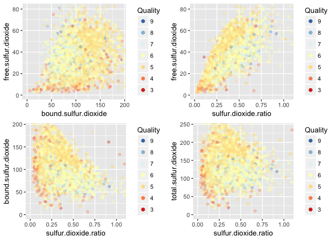
Sulfur dioxide
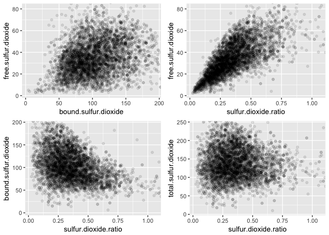
The sulfur dioxide ratio increases along with the free sulfur dioxide, and wines with greater ratios tend to have smaller concentrations of bound sulfur dioxide. I wonder how quality varies related to these variables.
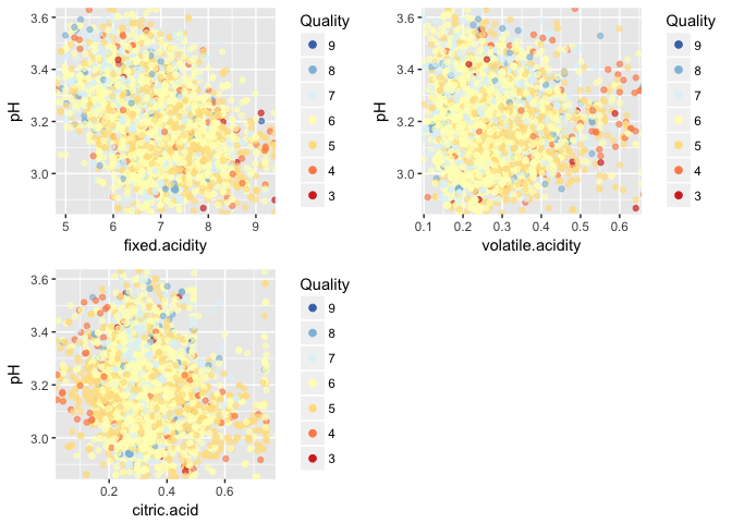
Acids
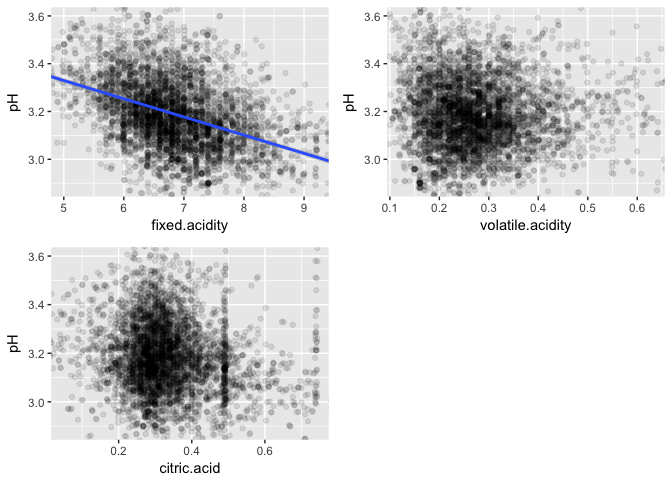
The only acid concentration that shows some considerable correlation with pH is the one regarding fixed acidity.
Main feature of interest: Quality
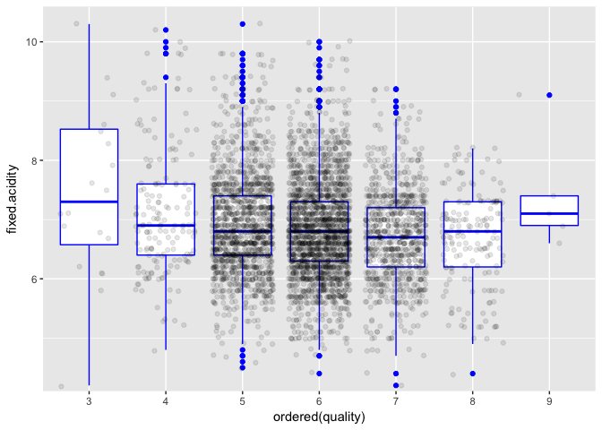
Better quality wines seem to have smaller fixed acidities on average.
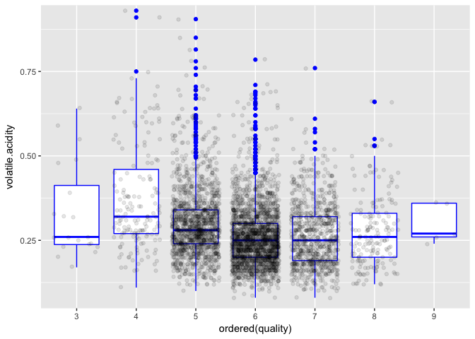
The same seems to apply with volatile acidity, but nothing very conclusive.
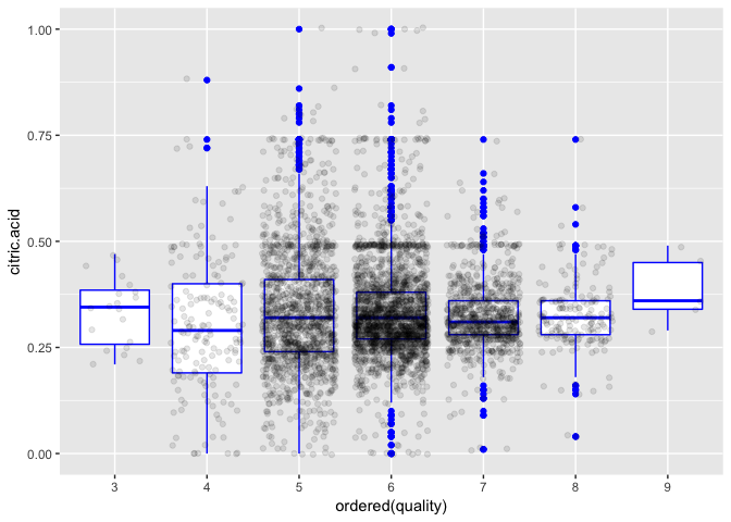
The low correlation on the panel above can be seen on these charts of quality by citric acid.
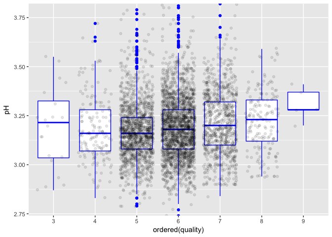
Except for wines with quality score 3, the median pH increases along with quality score.
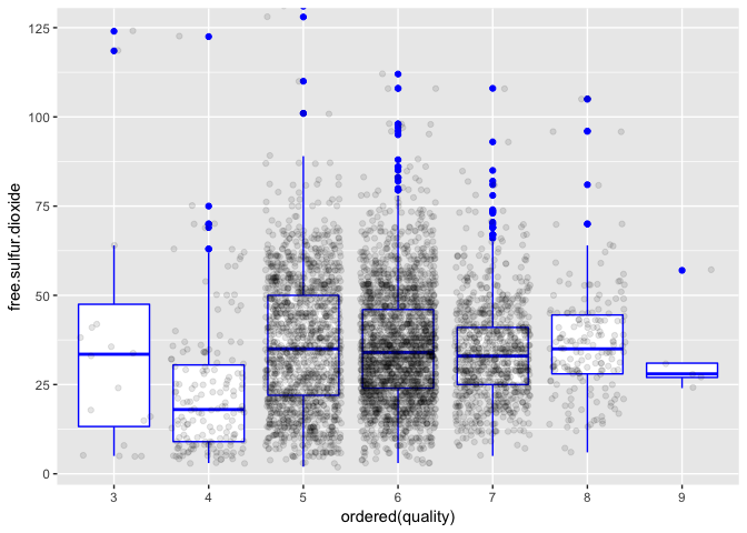
No clear relation between free sulfur dioxide and quality.
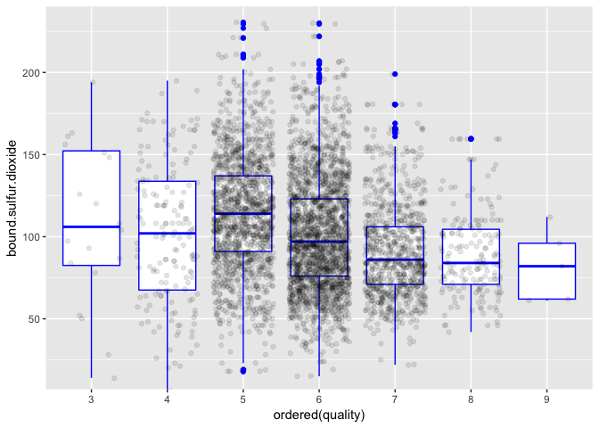
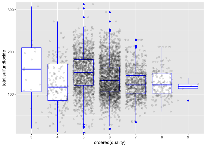
Here a trend can be seen. Overall, quality decreases as bound sulfur dioxide increases.
Here a slight correlation can be seen, somewhat similar to that of bound sulfur dioxide.
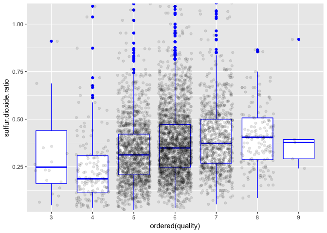
In general, quality increases as the ration of free and bound sulfur dioxide increases, but the correlation is weak.
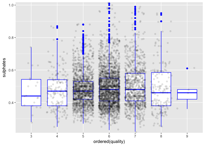
Sulphates don’t seem to add much isolatedly.
Nothing very clear from these charts.
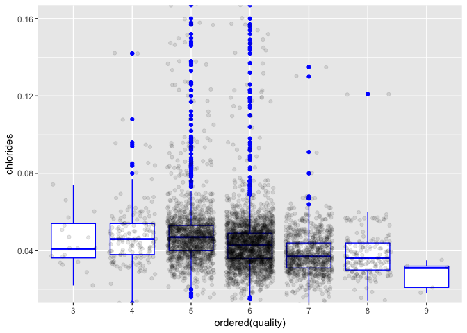
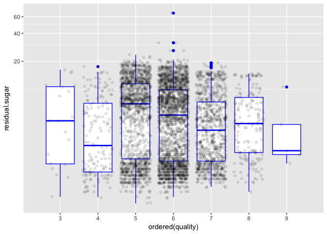
There is a curious amount of outliers for scores 5 and 6. I wonder why it happens.
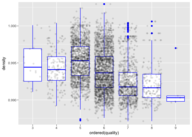
A greater correlation is more evident here. This seems to be one of the most promising relations so far. Maybe it has something to do with the fact that density is highly correlated with residual sugar and alcohol concentration, features that may be more easily detected by the experts palate.
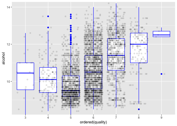
Alcohol is the variable with the greatest correlation with quality. It can be seen on the chart. Wines with grades 3 and 4 are going against the trend, but there are not many of those.
Bivariate Analysis
Talk about some of the relationships you observed in this part of the investigation. How did the feature(s) of interest vary with other features in the dataset?
I analyzed the relations between quality and every other variable in the dataset. The two largest Pearson’s correlations found were with alcohol (.436) and density (-.307). With both variables, an aproximately linear relation exsited for wines with scores from 5 to 9. The same did not apply for scores 3 and 4.
Analyzing the wines with quality score 9, I observed that they have in average a high concentration of alcohol, a very low density, and also a low amount of residual sugar. I imagine it derives from a well adjusted fermentation process, in which the sugar from the grapes is almost completely consumed in the process of fermentation, generating an above average alcohol concentration and thus a smaller density.
There is also a curious amount of outliers for scores 5 and 6. I wonder why it happens.
Did you observe any interesting relationships between the other features (not the main feature(s) of interest)?
Density is strongly correlated with two other variables: residual sugar (positively), and alcohol (negatively). It makes sense, taking into account the fermentation process of wine, in which sugar is consumed to generate alcohol. And since the residual sugar is more dense than alcohol, this inverse relation is presented.
Another relationship found was between fixed acidity and pH. Among the measures of acidity in the dataset, fixed acidity was the only one presenting at least a weak linear relationship with pH.
What was the strongest relationship you found?
The one between density and residual sugar. These features have a Pearson’s correlation coefficient of .839.
Multivariate Plots Section
I am dividing alcohol in bins to be able to plot density, alcohol, residual sugar and quality together and see how they relate with eachother:
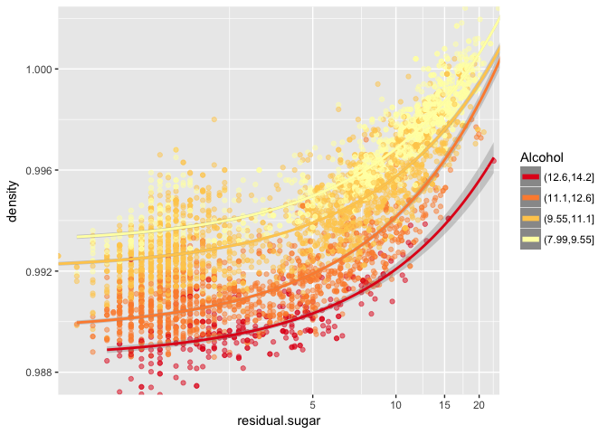
It can be seen that the points corresponding to higher amounts of alcohol show wines of better quality in average, and, for a given residual sugar, quality increases as density decreases.
Revisiting this chart from the bivariate plots section, but now colored by quality score. None of the charts indicate that this factors are well fit for a good linear model for predicting quality. However, some regions with higher concentrations of good and bad quality wines are defined, although not very clearly.
Revisiting this charts and adding quality as color, nothin very useful seemed to appear.
##
## Calls:
## m1: lm(formula = quality ~ alcohol, data = wines)
## m2: lm(formula = quality ~ alcohol + volatile.acidity, data = wines)
## m3: lm(formula = quality ~ alcohol + volatile.acidity + residual.sugar,
##     data = wines)
## m4: lm(formula = quality ~ alcohol + volatile.acidity + residual.sugar +
##     sulfur.dioxide.ratio, data = wines)
## m5: lm(formula = quality ~ alcohol + volatile.acidity + residual.sugar +
##     sulfur.dioxide.ratio + sulphates, data = wines)
## m6: lm(formula = quality ~ alcohol + volatile.acidity + residual.sugar +
##     sulfur.dioxide.ratio + sulphates + density, data = wines)
## m7: lm(formula = quality ~ alcohol + volatile.acidity + residual.sugar +
##     sulfur.dioxide.ratio + sulphates + density + pH, data = wines)
## m8: lm(formula = quality ~ alcohol + volatile.acidity + residual.sugar +
##     sulfur.dioxide.ratio + sulphates + density + pH + fixed.acidity,
##     data = wines)
## m9: lm(formula = quality ~ alcohol + volatile.acidity + residual.sugar +
##     sulfur.dioxide.ratio + sulphates + density + pH + fixed.acidity +
##     chlorides, data = wines)
## m10: lm(formula = quality ~ alcohol + volatile.acidity + residual.sugar +
##     sulfur.dioxide.ratio + sulphates + density + pH + fixed.acidity +
##     chlorides + citric.acid, data = wines)
##
## ===============================================================================================================================================
##                            m1         m2         m3         m4         m5          m6          m7           m8           m9           m10
## -----------------------------------------------------------------------------------------------------------------------------------------------
##   (Intercept)            2.582***   3.017***   2.356***   2.264***   2.014***   82.862***   102.754***   145.254***   143.910***   144.536***
##                         (0.098)    (0.098)    (0.114)    (0.114)    (0.125)    (12.567)     (12.925)     (18.216)     (18.506)     (18.561)
##   alcohol                0.313***   0.324***   0.375***   0.367***   0.368***    0.271***     0.242***     0.192***     0.192***     0.191***
##                         (0.009)    (0.009)    (0.010)    (0.010)    (0.010)     (0.018)      (0.019)      (0.024)      (0.024)      (0.024)
##   volatile.acidity                 -1.979***  -2.107***  -1.961***  -1.943***   -1.910***    -1.887***    -1.835***    -1.831***    -1.823***
##                                    (0.110)    (0.109)    (0.111)    (0.110)     (0.110)      (0.110)      (0.111)      (0.111)      (0.113)
##   residual.sugar                               0.027***   0.025***   0.026***    0.055***     0.065***     0.081***     0.081***     0.081***
##                                               (0.002)    (0.002)    (0.002)     (0.005)      (0.005)      (0.007)      (0.007)      (0.007)
##   sulfur.dioxide.ratio                                    0.384***   0.388***    0.319***     0.304***     0.308***     0.309***     0.308***
##                                                          (0.056)    (0.056)     (0.057)      (0.057)      (0.056)      (0.057)      (0.057)
##   sulphates                                                          0.463***    0.636***     0.588***     0.645***     0.644***     0.642***
##                                                                     (0.095)     (0.098)      (0.098)      (0.100)      (0.100)      (0.100)
##   density                                                                      -80.561***  -101.824***  -145.402***  -144.002***  -144.641***
##                                                                                (12.522)     (12.938)     (18.457)     (18.767)     (18.823)
##   pH                                                                                          0.472***     0.702***     0.695***     0.699***
##                                                                                              (0.076)      (0.103)      (0.105)      (0.105)
##   fixed.acidity                                                                                            0.068***     0.066**      0.065**
##                                                                                                           (0.020)      (0.021)      (0.021)
##   chlorides                                                                                                            -0.224       -0.251
##                                                                                                                        (0.543)      (0.546)
##   citric.acid                                                                                                                        0.043
##                                                                                                                                     (0.095)
## -----------------------------------------------------------------------------------------------------------------------------------------------
##   R-squared                 0.190      0.240      0.259      0.266      0.269      0.275        0.281        0.283        0.283        0.283
##   adj. R-squared            0.190      0.240      0.258      0.265      0.268      0.274        0.280        0.281        0.281        0.281
##   sigma                     0.797      0.772      0.763      0.759      0.758      0.754        0.752        0.751        0.751        0.751
##   F                      1146.395    773.875    568.789    442.368    360.295    309.623      272.891      240.632      213.878      192.478
##   p                         0.000      0.000      0.000      0.000      0.000      0.000        0.000        0.000        0.000        0.000
##   Log-likelihood        -5839.391  -5681.776  -5622.083  -5598.647  -5586.778  -5566.139    -5547.023    -5541.549    -5541.464    -5541.364
##   Deviance               3112.257   2918.264   2847.993   2820.870   2807.231   2783.672     2762.028     2755.862     2755.766     2755.653
##   AIC                   11684.782  11371.552  11254.166  11209.295  11187.556  11148.278    11112.045    11103.098    11104.927    11106.728
##   BIC                   11704.272  11397.538  11286.649  11248.274  11233.032  11200.250    11170.515    11168.064    11176.389    11184.687
##   N                      4898       4898       4898       4898       4898       4898         4898         4898         4898         4898
## ===============================================================================================================================================
Multivariate Analysis
Talk about some of the relationships you observed in this part of the investigation. Were there features that strengthened each other in terms of looking at your feature(s) of interest?
There is a very interesting relation between density, alcohol, residual sugar and quality. In general, quality increases as alcohol increases, density decreases and residual sugar decreases. These variables were amongst the most important predictors in the linear model built.
Were there any interesting or surprising interactions between features?
Since I did not have much knowledge of wine appraising before this exercise, I did not set expectations for the role of each variable, and therefore I was not surprised by the relations between them.
OPTIONAL: Did you create any models with your dataset? Discuss the strengths and limitations of your model.
I created a linear model for predicting quality. The R-squared value for the model was 0.283, which was a very low one. It indicates that a linear model probably is not the best fit for this dataset. Alcohol, volatile acidity and residual sugar were the most important prediction variables. Since there is a large correlation between some of the variables, some sort of feature selection would improve the model.
Final Plots and Summary
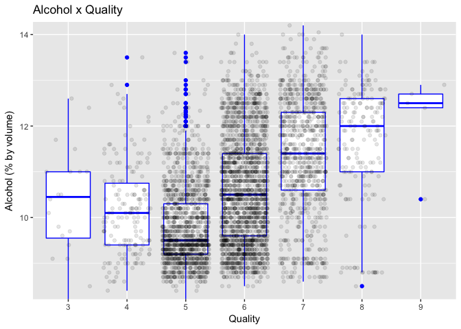
Plot One
Description One
This chart depicts the relation between alcohol concentration and quality score. For scores from 5 to 9, quality increases as alcohol increases, and for scores 3 and 4 the relation is the inverse. Alcohol has the largest correlation with quality among all the variables in the dataset, with a Pearson’s correlation coefficient of .436.
Plot Two
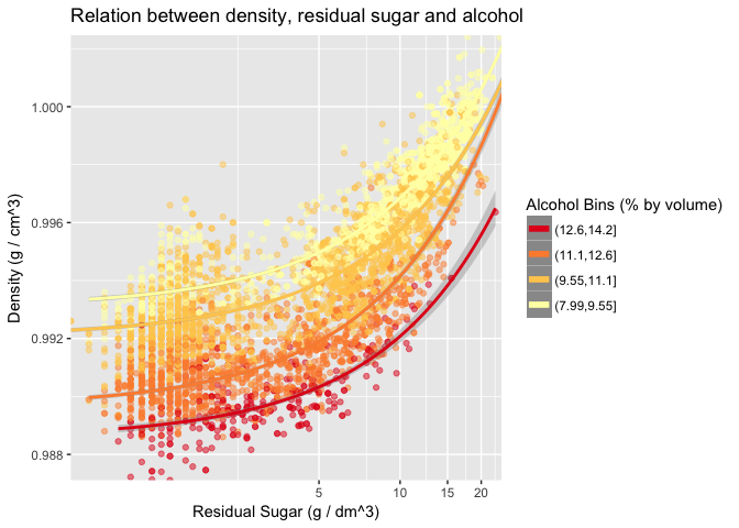
Description Two
A very interesting relation is shown in this chart. Given a value of residual sugar, density increases as alcohol decreases. This is in some extent due to the fermentation process of winemaking, in which sugar is consumed to generate alcohol. Since alcohol is less dense than water and sugar is more dense than water, this process makes the density of the wine decrease.
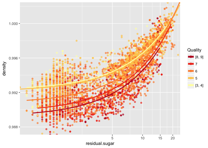
Plot Three
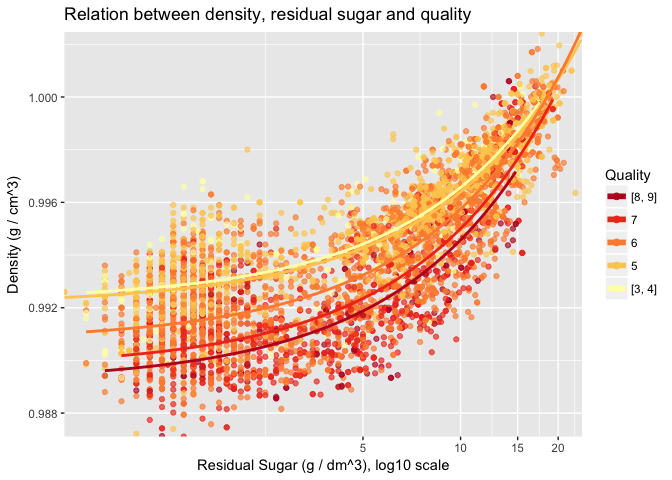
Description Three
This chart shows how quality relates with density and residual sugar. The two lowest and highest quality levels have been grouped to improve visibility.
It is noticeable that, for a given residual sugar concentration, quality increases as density increases. The same occurs if you fix density and increase residual sugar.
Reflection
This exploratory data analysis in which at first a univariate, then bivariate and finally multivariate examinations are performed allow for a progressive understanding of the dataset and the relations between its features.
Some interesting relations came up, like the one between alcohol, density, residual sugar and quality, that could be related to the fermentation process of wine. The correlation between pH and fixed acidity, while not correlating with volatile acidity and citric acids is also worth noting.
I strugled to find meaningful relations in the multivariate analysis section, and I have the feeling that some interesting relations may have been left aside among the many permutations of variables in the dataset. Anyway the whole analysis process was a very valuable experience, in which I practiced plotting various types of charts, handling overplotting and choosing the best chart type to convey the intended message.
A linear model for predicting quality was built, but it performed poorly, indicating that the dataset did not behave very much linearly. The process of evaluating wines is very subjective, and experts can be biased by their histories and preferences, making the relation between quality and the other variables too complex to be explained by a linear model. In the future, a diferent set of quality prediction models could be applied, and an evaluation of the best fit could be performed.
References
P. Cortez, A. Cerdeira, F. Almeida, T. Matos and J. Reis. Modeling wine preferences by data mining from physicochemical properties. In Decision Support Systems, Elsevier, 47(4):547-553. ISSN: 0167-9236. Available at: [@Elsevier] http://dx.doi.org/10.1016/j.dss.2009.05.016 [Pre-press (pdf)] http://www3.dsi.uminho.pt/pcortez/winequality09.pdf [bib] http://www3.dsi.uminho.pt/pcortez/dss09.bib